Classification
The
taxonomies used by
TROEPS
can be manipulated in order to find adequate places for objects and classes in
a given category or for building (upon particular criteria) a taxonomy from the
instances of the concept. Each functionality is presented in detail before
giving a complete example.
Instance
classification
Classification
is a suggestion mechanism, but instead of guessing the value of an object
field, it tries to find the possible classes for an object to migrate from its
current class to a lower (i.e. more specific) class. It is based on matching
the field values of the instance to be classified with the current candidate
class description. The classification takes place in each viewpoint along the
suitable hierarchy and uses bridges to jump from one class in a viewpoint to
another one in another viewpoint.
Starting
from the current belonging class of the instance in a given viewpoint, the
classification mechanism scans all of its subclasses and determines, for each
of them, if it is possible, unknown or impossible. A class is:
- possible
if the instance satisfies all the constraints on all the fields that exist in
this class;
- it
is unknown if no constraint in the class is violated, i.e. when the instance is
incomplete (with regard to the class specifications);
- it
is impossible if at least one constraint is not satisfied by a field value.
When
a class reveals itself impossible, all its sub-classes are labelled impossible
too. Thus, the algorithm iterates on every possible or unknown sub-classes, and
ends after it has reached the leaves of the hierarchy. When the classification
labels a class which is also the only source of a bridge, as possible or
unknown, it deduces that the destination class of the bridge (in another
viewpoint) is possible or unknown too. If this is not possible (because the
object does not satisfy the constraints of the destination), the initial object
is finally labelled as impossible
.
The
function provided below constitutes the minimal classification service in
TROEPS.
Improvements are planned including:
- the
interactive querying of the user for unknown values (with, if possible, clever
algorithms);
- taking
into account exclusive, exhaustive and definitional nature of the taxonomies;
- better
algorithm for classification cache;
- taking
into account recursive objects.
Interface

Screendump
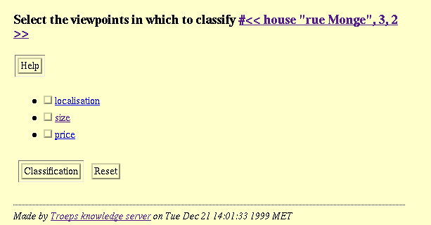
46: Classification initialisation.

Screendump
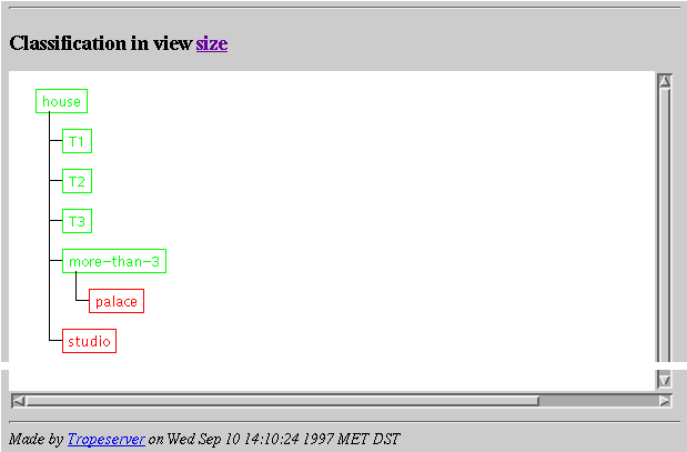
47: Classification result. Classes are displayed in either red (impossible),
yellow (unknown) or green (possible). As a result of classification, clicking
on a class will access to that class while when used in attach query (see
Screendump
32
),
it will attach the object to the selected class.
API
- (tr-classify
object rest: views
) function
in [libtrp]
-> ( ( ( class* ) ( class* ) . ( class* ) )* ),
object
object
nao,views
{ conceptview
nakv*
}
ivsp
- Returns,
for each of the provided concept viewpoints
views
-- and if none is provided, for each of the views of the concept --, the sets
of possible, unknown and impossible classes for the object
object.
- (tr-attachable
object
class) function
in [libtrp]
-> symbol: {imp, unk, pos},
object
object
nao,class
class
nac,ivc
- Returns
a value among
pos,
unk
and
imp
indicating if the object
object
is attachable to the class
class.
Note that if the class
class
is not a subclass of the current object class under the concept, the returned
value is
imp.
Examples

Figure
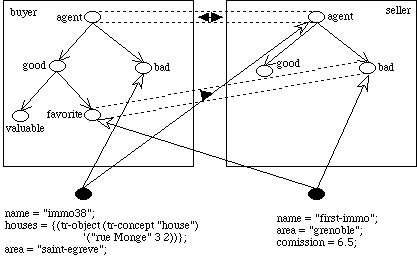
11: At the end of the complete example session, the resulting situation is
presented here.
? (tr-classify (tr-object (tr-concept "agent") '("first-immo")))
= ((((tr-class (tr-conceptview (tr-concept "agent") "buyer") "favorite"))
    ())
   (((tr-class (tr-conceptview (tr-concept "agent") "seller") "bad"))
    ()))
? (tr-classify (tr-object (tr-concept "agent") '("immo38")))
= ((((tr-class (tr-conceptview (tr-concept "agent") "buyer") "bad"))
    ())
   (((tr-class (tr-conceptview (tr-concept "agent") "seller") "agent")
     (tr-class (tr-conceptview (tr-concept "agent") "seller") "bad")
     (tr-class (tr-conceptview (tr-concept "agent") "seller") "good"))
    ()))
? (tr-attachable
    (tr-object (tr-concept "agent") '("immo38"))
	 (tr-class (tr-conceptview (tr-concept "agent") "buyer") "good"))
= imp
? (tr-attachable
    (tr-object (tr-concept "agent") '("immo38"))
	 (tr-class (tr-conceptview (tr-concept "agent") "buyer") "bad"))
= pos
? (tr-attachable
    (tr-object (tr-concept "agent") '("immo38"))
	 (tr-class (tr-conceptview (tr-concept "agent") "buyer") "agent"))
= pos
? (tr-attachable
    (tr-object (tr-concept "agent") '("immo38"))
	 (tr-class (tr-conceptview (tr-concept "agent") "seller") "good"))
= pos
? (tr-attachable
    (tr-object (tr-concept "agent") '("first-immo"))
	 (tr-class (tr-conceptview (tr-concept "agent") "buyer") "good"))
= pos
Categorisation
Categorisation
consists in inferring the possible positions, in a taxonomy, for a particular
class definition. This capability is not provided yet.
Clustering
Clustering
consists in organising a set of objects into one or several taxonomies.
Clustering methods divide the set of objects into previously unknown classes
whereby the main principle may be summarized as follows : the most similar
objects are put in the same class and the less similar ones in distinct
classes. A function of proximity is used to evaluate the likeness degree of
pair of objects. In
TROEPS,
the clustering facility is based on a universal dissimilarity among the objects
manipulated by the system, it can therefore cluster the objects of any concept
and return the result as a taxonomy of intensionnally described classes. An
environment to host various methods for automatic taxonomy construction,
T-TREE,
is included in
TROEPS.
A
detailled account of clustering is given here. However, it can be summarised as
follows:
- determine
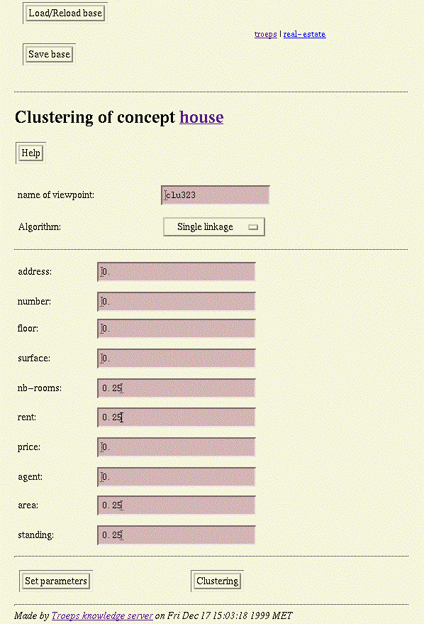
the concept to cluster and provide the weights for the fields on which the
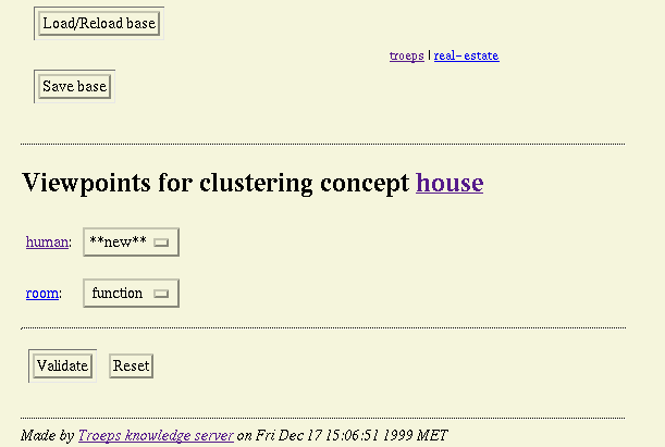
dissimilarity will be computed (see
Screendump
48
);
- T-TREE
will ask how to compute dissimilarity on objects of concepts which are the type
of selected fields. This can be done either by using a particular viewpoint or
by choosing to cluster this concept (see
Screendump
49
).
In the second event, step 1 will be called again;
- T-TREE
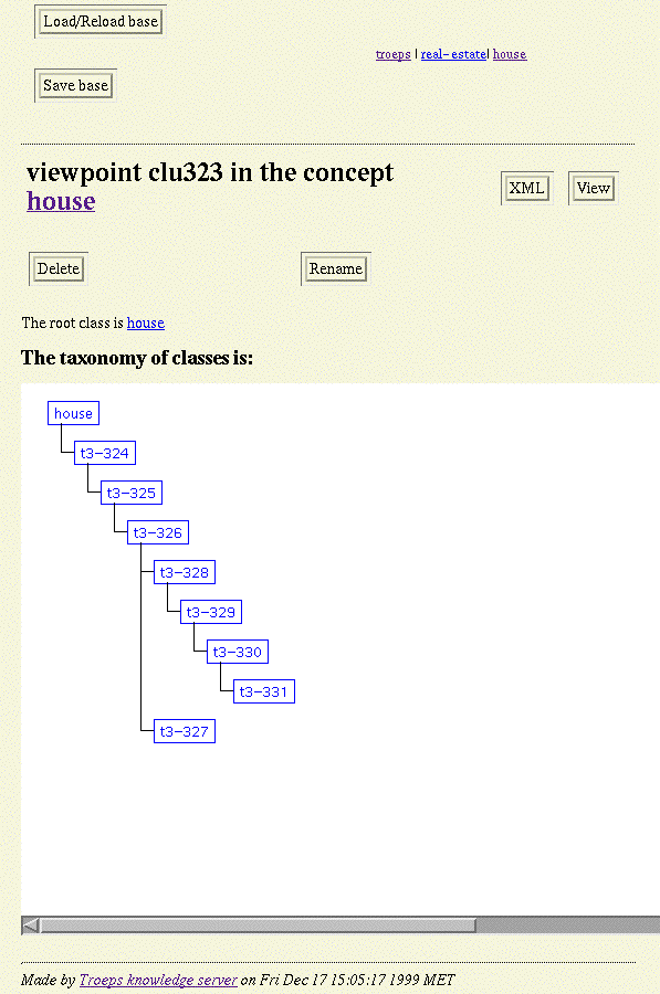
returns the computed cluster, i.e. a new viewpoint with a class taxonomy (see
Screendump
50
).
For
performing this, the system will, for each viewpoint, in a relevant order,
compute the dissimilarity between each pair of objects of the concept. This
will depend on the dissimilarity between their field values and the weights
applied to field by the dissimilarity measure. Then, the system will aggregate
objects into sets (the most similar objects first) and the sets will be
aggregated into supersets (forming a taxonomy). Last, all these sets will be
provided by class descriptions. This is the resulting taxonomy.
Dissimilarity
The
aim of a proximity measure is to evaluate to what extent a pair of objects are
alike (or unlike) with respect to the available information about them. Within
an object model this information may be extracted either from object fields
values or from the class taxonomy of the underlying concept (the mutual
position of objects within the taxonomy).
In
both cases the comparison of a pair of objects takes advantage of the
fundamental principle of the object paradigm, which is the hierarchical
organisation of the manipulated entities. Thus, the
T-TREE
built-in dissimilarity measure, called
topological,
is based on the fundamental principle of the object paradigm: organising the
manipulated entities in a hierarchical manner. It relies on universally
available relationships: sub-typing and class specialisation.
For
a given pair of objects, the topological dissimilarity is computed with respect
to their field values. First, a field-level function computes the differences
between the respective pairs of field values. Then, an object-level function
combines the values computed in this way into a single global result that
caracterizes the compared objects.
The
contribution of a field to the global dissimilarity value depends on the nature
of the field domain. For abstract data types, i.e. primitive value domains,
this contribution is computed on the hierarchical structure of meaningful
sub-domains. In fact, given a pair of values, their dissimilarity is based on
the relative
size
of their smallest common sub-domain. The size of a (sub-)domain is the number
of domain values it includes. Thus the size of an integer interval [0 2] is 3
as there are three values, 0, 1, and 2. Surprisingly, when taken over an
integer domain, the interval [1 1] is of size 1, whereas on a real one its size
is 0. This rather complex way of computing the value dissimilarity has the
advantage of being universally applicable on simple data types.
In
fact, each basic data type connected to
TROEPS
(see Appendix
5)
is provided with a function computing this value. Furthermore, the generic
function, when applied on some standard types like integers, reals, etc.
matches the well-known and mostly used distance functions like the arithmetic
difference on integers.
For
instance, given the three objects of the house concept presented in the
following table:
|
objects
\ fields
|
address
|
number
|
floor
|
|
house-1
|
"grenoble"
|
113
|
0
|
|
house-2
|
"grenoble"
|
21
|
2
|
|
house-3
|
"eybens"
|
13
|
4
|
The
topological dissimilarity will compare them with respect to the values of a
previously selected sub-set of fields. For instance, if one chooses to use the
address,
the
floor
and the
number
fields, whereby their relative importance (or weights) are 0.5, 0.2 and 0.3
respectively, the following computation can be done.
First,
the elementary distance between
house-1
and
house-2
with respect to the
address
field is 0, since the field type, string, is of unordered (nominal) type
family. Thus, only identical items lead to a 0 value for the difference whereas
in other cases that value is 1. Furthermore, the address field differences
score to a 1 for both the pairs (
house-1,
house-3)
and (
house-2,
house-3).
The remaining two fields are processed, in a similar way. The specific point
with
floor
and
number
is that their types are numeric (quantitative) and discrete. so the arithmetic
difference is taken and a normalisation is performed on it. Starting with the
difference on
floor
for (
house-1,
house-2),
one first computes their most specific common interval which is [0 2] and
corrects it by 1 (the mean of the sizes of [0 0] and [2 2], both scoring to
1). The remaining value is divided by 4, the size of the whole domain which
yields 0.5. This exactly corresponds to the normalized arithmetic difference on
[0 4].
Thus,
during clustering, the dissimilarity between two objects can be computed by
aggregating the dissimilarities with regard to each field. Precisely, the
dissimilarity between each field value is computed (by the previous method) and
a weighted combination of each measure is computed (weights are provided through
Screendump
48
). For
instance, the weighted sum (weighted City block function) of the example above
will compute the following values:
d(house-1,
house-2)
= 0.5 * 0 + 0.2 * 0.5 + 0.3 * 0.92 = 0.1 + 0.276 = 0.376,
d(house-1,
house-3)
= 0.5 * 1 + 0.2 * 1 + 0.3 * 1 = 0.5 + 0.2 + 0.3 = 1,
d(house-2,
house-3)
= 0.5 * 1 + 0.2 * 0,5 + 0.3 * 0.08 = 0.5 + 0.1 + 0.024 = 0.624.
The
same principle is applied on object-valued fields: the likeness between objects
taken as field values depends on their respective positions within the
underlying taxonomy. Actualy, a taxonomy provides a set of classes which
represent the admissible sub-domains of the whole object domain which is itself
defined by the underlying concept. The dissimilarity is measured on the most
specific common super-class of both objects. The number of the member objects
is taken as class size. Thus, the most specific the common class, the most
similar the member objects. Besides, the same computation procedure, i.e.
corrections and normalization, applies on both objects and simple values.
For
instance, on
Figure
13
,
the following inter-object dissimilarities may be computed :
d(house-1,
house-2)
= 0.4,
d(house-1,
house-3)
= 1,
d(house-2,
house-3)
= 0.6.
The
topological measure allows the various aspects of the concerned objects to be
taken into account: the resemblance of objects under different viewpoints are
evaluated separately (in function of the length of the shortest path between
them in the taxonomy) and then aggregated to a single, usually weighted, mean.
In both cases, i.e. primitive value domains and object sets, the result of the
field-level dissimilarity function is real number between 0 and 1.
The
above computation clearly requires the presence of at least one meaningful
taxonomy over the concerned concept. In some cases, however, it is impossible
to ensure the availability of classes, especially when the whole process is
aimed at class discovery. Therefore, the comparison of objects remains only
possible with respect to their field values. In such cases,
T-TREE
applies the same dissimilarity function as on initial objects, i.e. a weighted
City block distance. It also applies clustering in order to better characterise
the domains of the fields of the initial concept.
A
technique of this kind may lead, when some circuits in object definitions
occur, to a deadlock between dissimilarity computation tasks. In fact, it may
happen that the dissimilarity of a pair of objects depends on the dissimilarity
of another pair which in turn depends on the first dissimilarity. In such a
case, a fixed point computation is applied in order to simultaneously evaluate
the proximity of all mutually dependant pairs. The definitions of the
dissimilarity on each pair is used to extract characterization functions which
further compose a system of equations. The underlying vector function is
repeatedly applied on an initial solution until a suitable approximation of the
function fixed point is obtained. Its components represent approximations of
the dissimilarities saught.
Clustering
algorithms
Several
algorithms of the Sequential Agglomerative Hierarchical Non-overlapping familly
are currently available (complete, single -- a.k.a. nearest neighbours --,
average linkage). They can be characterised as ascending binary clustering
algorithms (which progressively aggregate classes, starting from the instances,
and only aggregate two classes in a row). The algorithms begin by considering
each object as a class. Then, at each step, they aggregate into a new class the
two classes which contains the nearest objects with regard to the dissimilarity
measure. This new class contains the objects of the two previous ones which are
not considered further. The algorithm stops when there is only one class left.
Based
on the above values, a clustering algorithm will try to divide the set of
objects into homogeneous sub-sets. I.e., object groups will be looked for such
that the member objects score to low values of the pairwise dissimilarity
whereas the pairs of objects in different groups score to higher values. In the
example, a sub-group will be created including
house-1
and
house-2
since
their dissimilarity, 0.376, is substantially lower than the one of the pairs (
house-1,
house-3)
and (
house-2,
house-3).
Thus two classes will be generated
c1
and
c2,
having extensions {
house-1,
house-2,
house-3}
and {
house-1,
house-2}
respectively. In other terms,
c2
is a sub-class of
c1.
Generalisation
The
result of the clustering phase is an inclusive hierarchy of sets of objects. In
order to provide a description corresponding to these sets, a class description
is inferred from each set of objects provided. The details of the
generalisation mechanism provided are not described here. However, the
application of the generalisation procedure on above example yields the
following partial class descriptions:
<c1
	fields = {
		<address domain = {"eybens", "grenoble"};>,
		<number intervals = {[13 113]};>,
		<floor intervals = {[0 4]};>};>
<c2
	superclass = c1;
	fields = {
		<address domain = {"grenoble"};>,
		<number intervals = {[21 113]};>,
		<floor intervals = {[0 2]};>};>
Interface

Screendump
48: Clustering initialisation.

Screendump
49: Object dissimilarity completion.

Screendump
50: Clustering result.

Screendump
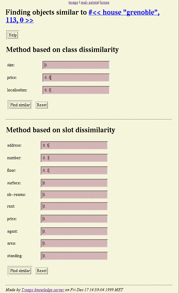
51: Dissimilarity initialisation.

Screendump
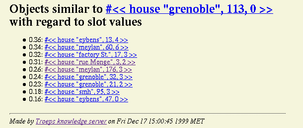
52: Dissimilarity result.
API
- (tr-clustering
concept
method
create-p viewname slots
) function
in [libtrt]
-> (),
concept
concept
nak,method
string
nas,
create-p
boolean,
viewname
string
nas,adkv
,
slots
( (conceptslot
naks
. float
bcf)
nal
*)
nal
- Builds
a new taxonomy of classes for concept
concept
in a viewpoint called
viewname
(which is created if
create-p
is not
())
by considering only the slots in
slots
with their respective weight comprised between
0.
and
1..
The method used for clustering depends on the first element of the
method
argument (available methods are
"mv",
"al",
"sl"
and
"cl").
This
API function works perfectly for fields whose type is not another concept. In
the opposite event, each such classslot must be created and the
clview
annotation set to the name of the concept view (of the domain concept) to use.
This view must have been created. Either, it already has a taxonomy which is
then used or it has class fields in its root class whose
clweight
annotation is set to a weight and
clalgo
whose value is the name of an algorithm as above and this recursively.
- (tr-find-slot-similar
object
slots) function
in [libtrt]
-> ((object . float)*),
object
object
nao,
slots
( (conceptslot
naks
. float
bcf)
nal
*)
nal
- Compare
the object
object
with all the other instances of its concept on the basis of the set
slots
of fields weighted by floats between 0. and 1. (whose sum is 1.) and returns
their list ordered by higher similarity. This uses the weighted agglomeration
of the dissimilarity between the concerned field values.
- (tr-find-view-similar
object
views) function
in [libtrt]
-> ((object . float)*),
object
object
nao,
views
( (conceptview
nakv
. float
bcf)
nal
*)
nal
- Compare
the object
object
with all the other instances of its concept on the basis of the set
views
of views weighted by floats between 0. and 1. (whose sum is 1.) and returns
their list ordered by higher similarity. This uses the weighted topological
dissimilarity over the concerned views.
Examples
Bridge
inference
Once
taxonomies have been built and objects have been attached, it is very
convenient to be able to compare them. To that extent, bridge inference
algorithms are provided which produce bridges holding between the classes of
the taxonomies.
The
algorithms are used from a set of classes and a class and they look for all the
bridges which involve subclasses of the former as source and subclasses of the
latter as destination. The algorithms compare the classes and if all the
"conjunction" of the source classes is smaller than the destination classes.
However, it only returns the minimal bridges in the meaning provided in the
Bridge section. So, the user can choose to implement a non minimal bridge. But
any bridge not covered by a bridge returned by the algorithm is not valid.
There
are two versions of the algorithm depending on the predicates they rely on. A
first version uses the members of the classes such that conjunction is
intersection of these member sets and comparison is inclusion; the second
version uses the types of the classes such that conjunction is type
intersection and comparison is a sub-typing test.
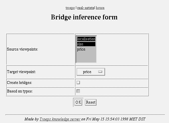
Interface

Screendump
53: Bridge inference initialisation.

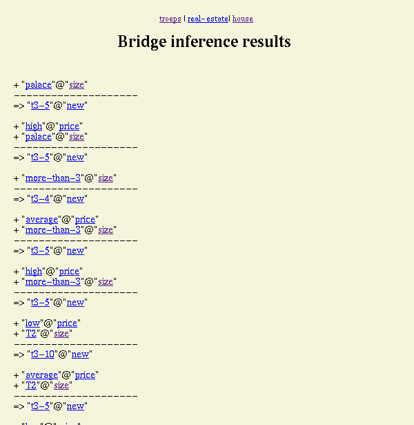
Screendump
54: Bridge inference result.
API
-
(
tr-find-bridges-from-objects
classes
class
create-p
) function
in [libtrt]
-> { ( (class*) . class)* },
classes
class
nas,class
class
nac,ivc,
create-p
boolean
- Looks
for all the minimal possible bridges which have a subset of subclasses of
classes
as source and a subclass of
class
as destination. The possibility of a bridge is judged with regard to the set of
objects members of each class. The bridges are created if
create-p
evaluates to true, their compositions are returned otherwise.
- (tr-find-bridges-from-types
classes
class
create-p
) function
in [libtrt]
-> { ( (class*) . class)* },
classes
class
nas,class
class
nac,ivc,
create-p
boolean
- Looks
for all the minimal possible bridges which have a subset of subclasses of
classes
as source and a subclass of
class
as destination. The possibility of a bridge is judged with regard to the type
of each class. The bridges are created if
create-p
evaluates to true, their compositions are returned otherwise.
Examples
Complete
example
Let
the set of objects be the one contained in the real-estate knowledge base
provided in the example directory. The set of 10 objets is given below with the
relevant slot values:
|
#
|
address
|
number
|
floor
|
area
|
standing
|
nb-rooms
|
rent
|
|
1
|
factory
St
|
17
|
3
|
grenoble
|
fair
|
4
|
6000.
|
|
2
|
meylan
|
176
|
3
|
meylan
|
fair
|
3
|
8000.
|
|
3
|
smh
|
95
|
3
|
smh
|
low
|
1
|
3000.
|
|
4
|
grenoble
|
113
|
0
|
grenoble
|
low
|
2
|
4000.
|
|
5
|
meylan
|
60
|
6
|
meylan
|
high
|
4
|
11000.
|
|
6
|
eybens
|
47
|
0
|
eybens
|
fair
|
2
|
7000.
|
|
7
|
eybens
|
13
|
4
|
eybens
|
fair
|
8
|
11000.
|
|
8
|
grenoble
|
21
|
2
|
grenoble
|
low
|
3
|
8000.
|
|
9
|
grenoble
|
32
|
3
|
grenoble
|
high
|
5
|
14000.
|
|
10
|
rue
Monge
|
3
|
2
|
paris
|
fair
|
2
|
15000.
|
These
object are first classified and attached to the most non ambiguous specialised
class (i.e. the lowest class to which the objects can be attached while they
cannot be attached to a non comparable class). For instance, the house #4 is
attached to
other-area
while it can be attached to both
industrial
and
residential.
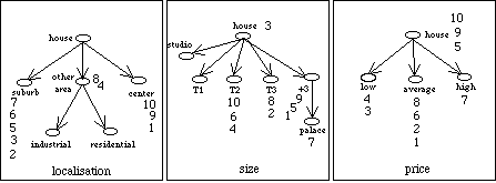
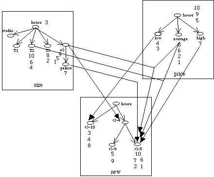
The result is given in the table below and in
Figure
12
.
It is noteworthy that object 5, 9 and 10 are not attached to
high
under the
price
viewpoint because of a bridge stating that the high priced houses are palaces
(that which these houses cannot pretend to be since they have at most 3 rooms).
On the contrary, house #7 is attached to
high
because it can be attached to
palace.
|
#
|
localisation
|
size
|
price
|
new
|
|
1
|
center
|
More
than 3
|
average
|
t3-5
|
|
2
|
suburbs
|
T3
|
average
|
t3-5
|
|
3
|
suburbs
|
H
|
low
|
t3-10
|
|
4
|
other-area
|
T2
|
low
|
t3-10
|
|
5
|
suburbs
|
More
than 3
|
house
|
t3-9
|
|
6
|
suburbs
|
T2
|
average
|
t3-5
|
|
7
|
suburbs
|
Palace
|
high
|
t3-5
|
|
8
|
other-area
|
T3
|
average
|
t3-10
|
|
9
|
center
|
More
than 3
|
house
|
t3-9
|
|
10
|
center
|
T2
|
house
|
t3-5
|

Figure
12: The various viewpoints and the attached objects after classification.
A
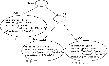
new viewpoint is created by clustering on the slots
area,
standing,
nb-rooms
and
rent
with the same .25 weight. Interesting resulting classes are provided in
Figure
16
.
It retains only the upper classes (the other ones have been discarded -- that
which, as like as renaming classes, is easily done with the graphic user
interface). It can be noted that only one field (
standing)
allows to discriminate the classes. This is due to the importance of the
dissimilarity between different nominal values. Overall, the classes t3-10 and
t3-9 corresponds to two homogeneous groups (they can be independently
discriminated by the
standing,
rent
and
nb-rooms
fields.

Figure
13: Interesting classes in the new viewpoint.
Last,
it is possible to call the bridge inference methods in order to investigate the
correlation between classes of different viewpoints.
Figure
14
displays the result when using the inference from objects between viewpoints
size, price and the newly created viewpoint.

Figure
14: Bridge inference based on objects. Here are all the maximal bridges which
do not target the root class.
